FBref - Pressures
Using FBref data to looking to team/league pressing habits

I haven’t put anything together for a while at my blog but will slowly migrate everything over to here! Since I first put something together last year I get regular questions/requests…this is one of those!
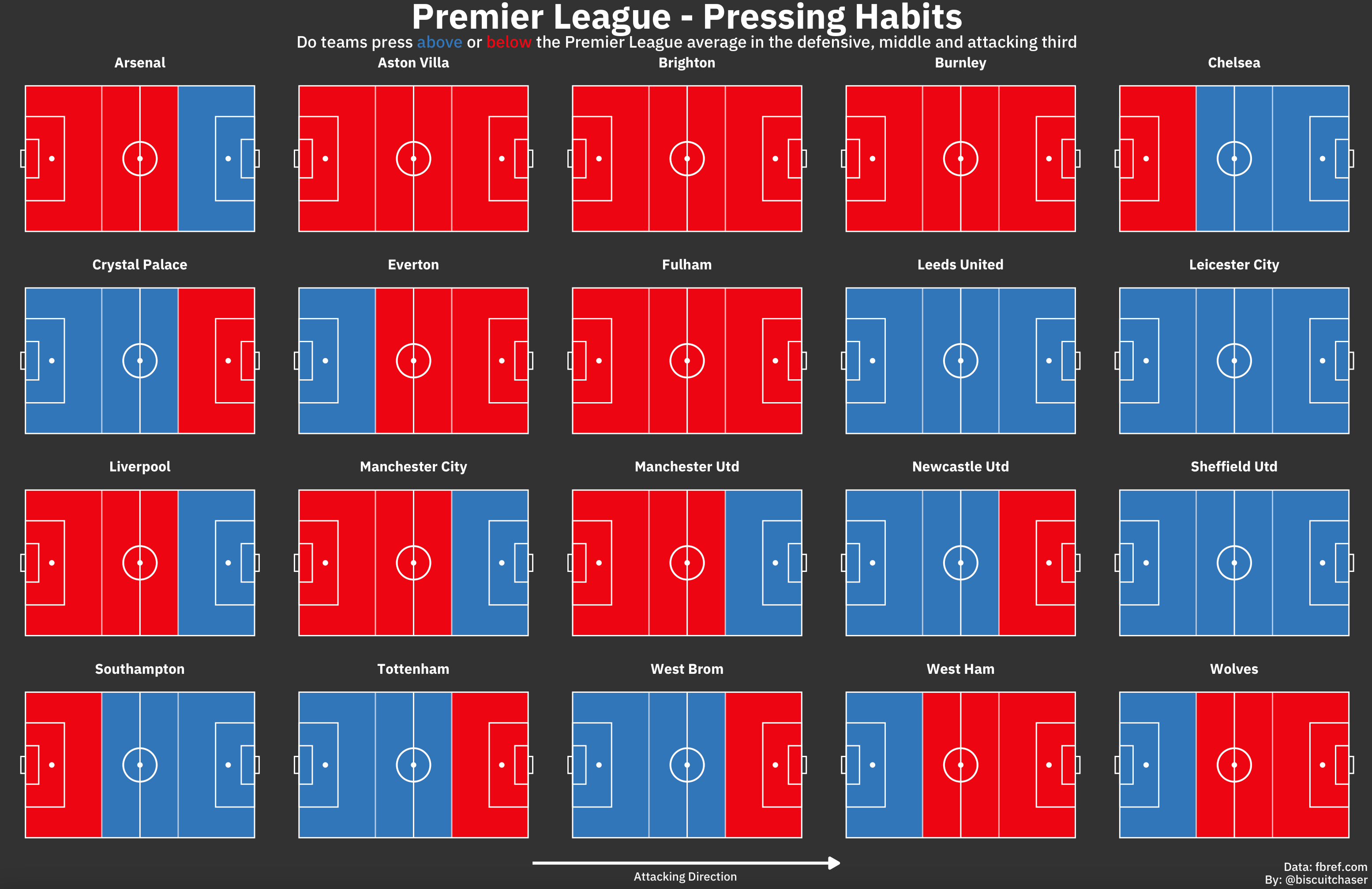
Anyway, this is what we are aiming for:
I suspect this will become the start of something larger investigating pressing habits, but we will see how it goes!
We will be using StatsBomb data via FBref - we can pull the data using the worldfootballR package. The packages required:
library(worldfootballR)
library(ggsoccer)
library(ggtext)
library(RColorBrewer)
library(glue)
library(cowplot)
library(janitor)

##to install worldfootballR
devtools::install_github("JaseZiv/worldfootballR")
I will also use an amended pitch from ggsoccer as when the fill is set to transparent, as we will require, the result is this:

To pull the defensive stats for the top 5 European Leagues for 2020/2021 we can run:
##get defensive stats for big 5 European Leagues and clean headers

df <- get_season_team_stats(country = c("ENG", "ESP", "ITA", "GER", "FRA"), gender = "M", season_end_year = 2021, stat_type = "defense") %>%
janitor::clean_names()

head(df)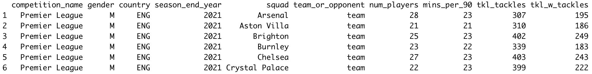
The next chunk will group the data, apply some summary stats then select the columns we wish to keep and filter:
##nest by league and run mean pressures in def/mid/att 3rds - select and filter by single league

data<-df %>%
  group_by(country, team_or_opponent) %>%
  nest() %>%
  mutate(def_av = map(.x = data, ~mean(.x$def_3rd_pressures)),
         mid_av = map(.x = data, ~mean(.x$mid_3rd_pressures)),
         att_av = map(.x = data, ~mean(.x$att_3rd_pressures))) %>%
  unnest() %>%
  select(competition_name,country, team_or_opponent, squad, def_3rd_pressures:att_3rd_pressures, def_av:att_av) %>%
  filter(country=="ENG",
         team_or_opponent=="team")
Above I have only selected the “team” element rather than the behaviour of the opponent…although that offers another rabbit hole to get lost down!
Now to set some stuff up for the plot:
##league name
league<-unique(data$competition_name)

##set season
season_name<-"2020/2021"

##check colourblind palettes and select hex
display.brewer.all(colorblindFriendly = TRUE)
brewer.pal(n=11, "RdYlBu")

colour_1<-"#4575B4"
colour_2<-"#D73027"
colour_3<-"grey97" ##font colour

##coords for dividing pitch into thirds
lines<-tibble(x = c(33.33, 66.66),
              y = 0,
              xend = c(33.33, 66.66),
              yend = 100)
The beauty of ggplot is that we can build in layers - here comes the gradual plotting!
ggplot()+

  geom_rect(data = data, aes(xmin = 0, xmax = 33.33, ymin = 0, ymax =100), fill = ifelse(data$def_3rd_pressures>data$def_av, colour_1, colour_2))+

  geom_rect(data = data, aes(xmin = 33.33, xmax = 66.66, ymin = 0, ymax =100), fill = ifelse(data$mid_3rd_pressures>data$mid_av, colour_1, colour_2))+

  geom_rect(data = data, aes(xmin = 66.66, xmax = 100, ymin = 0, ymax =100), fill = ifelse(data$att_3rd_pressures>data$att_av, colour_1, colour_2))+

  geom_segment(data = lines, aes(x = x, y = y, xend = xend, yend = yend), colour = colour_3, alpha = 0.6)
The above looks scary if you haven’t done much coding previously, however the 3 geom_rect elements are diving the pitch into thirds, using ifelse to conditionally fill. (The ifelse reads if data$def_3rd_pressures is greater data$def_av colour_1 (if true), colour_2 (if false).
The output should look something like this:

The next part will call the transparent filled pitch:
annotate_pitch_one(colour = colour_3, fill = "NA")+
  theme_pitch()
Starting to get a little closer to what we are after! Finally will call facet_wrap(~squad) to gain an overview of all EPL teams:
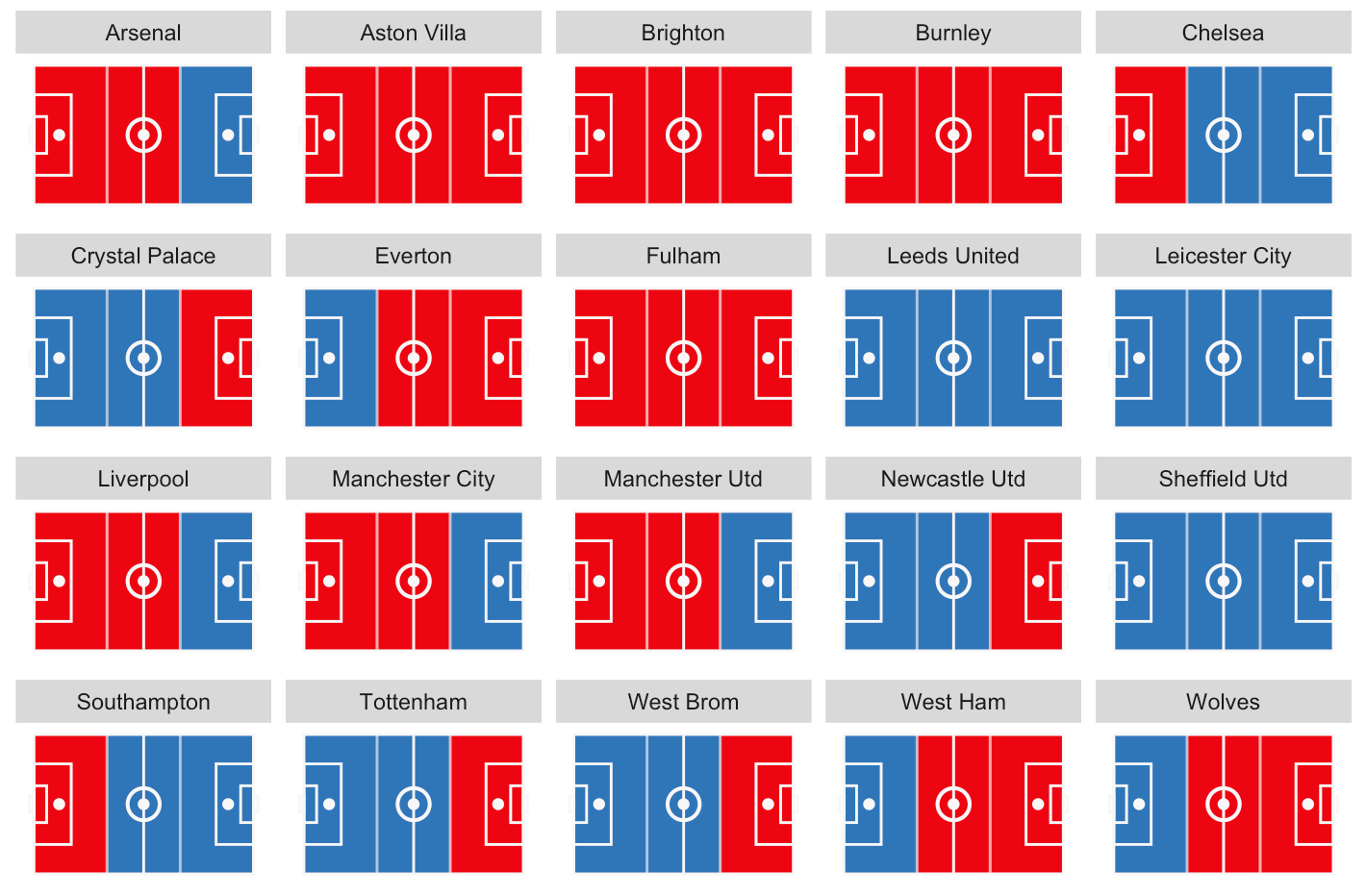
At this point the code should look something like:
ggplot()+

  geom_rect(data = data, aes(xmin = 0, xmax = 33.33, ymin = 0, ymax =100), fill = ifelse(data$def_3rd_pressures>data$def_av, colour_1, colour_2))+

  geom_rect(data = data, aes(xmin = 33.33, xmax = 66.66, ymin = 0, ymax =100), fill = ifelse(data$mid_3rd_pressures>data$mid_av, colour_1, colour_2))+

  geom_rect(data = data, aes(xmin = 66.66, xmax = 100, ymin = 0, ymax =100), fill = ifelse(data$att_3rd_pressures>data$att_av, colour_1, colour_2))+

  geom_segment(data = lines, aes(x = x, y = y, xend = xend, yend = yend), colour = colour_3, alpha = 0.6)+

  annotate_pitch_one(colour = colour_3, fill = "NA")+

  theme_pitch() +

  facet_wrap(~squad)
From this point is the customisation - starting with the labels:
labs(title = glue("{league} - Pressing Habits {season_name}"),
       subtitle = glue("<b style='color:grey97'>Do teams press </b><b style='color:#4575B4'>above </b><b style='color:grey97'>or </b><b span style='color:#D73027'>below </b><b style='color:grey97'>the {league} average in the defensive, middle and attacking third?</b>"),
       caption = ("Data: fbref.com
                  By: @biscuitchaser"))
The above sets our title/subtitle and caption using the ggtext package to add a legend colouring to the text.
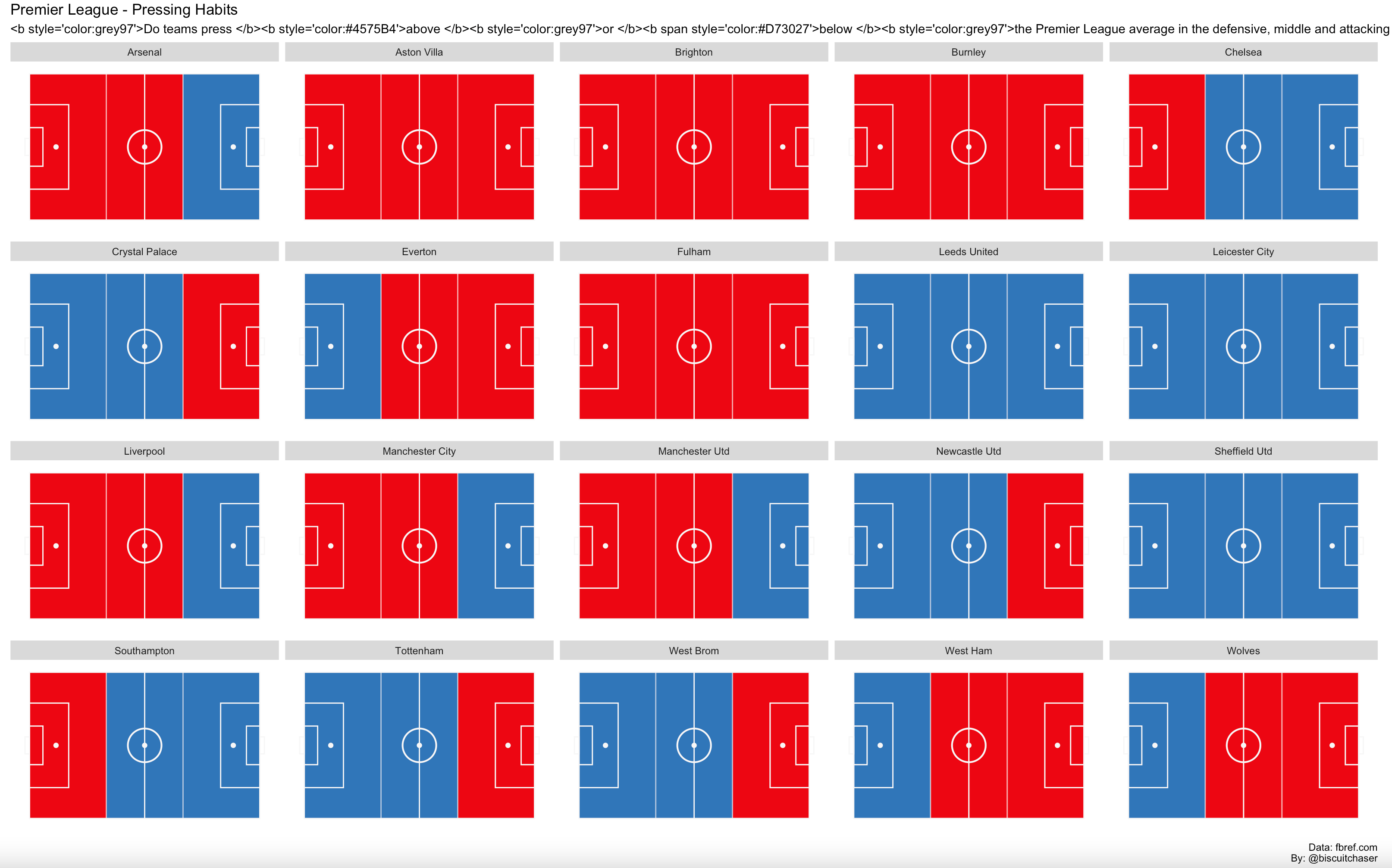
The subtitle is chaos at the minute, but this will change once we introduce the theme() elements and element_textbox_simple():
theme(plot.title = element_textbox_simple(size = 30, colour = colour_3, face = "bold", halign = 0.5),

plot.subtitle = element_textbox_simple(size = 14, halign = 0.5),

plot.caption = element_text(size=10, colour = colour_3),

legend.position = "none",

plot.background = element_rect("grey20"),

strip.background = element_blank(),

strip.text = element_text(colour = colour_3, size = 12))
The above should be pretty straightforward but within the above have
dealt with the plot title/subtitle and caption
removed the plot legend
set the background fill (I find the black/white contrast to be too harsh so use grey20 and grey97 for the font…feels softer on the eyes but is all personal preference!)
remove the facet label background and set the text
Finally assign the plot as we will use it for the final edit!
p<-ggplot()+

  geom_rect(data = data, aes(xmin = 0, xmax = 33.33, ymin = 0, ymax =100), fill = ifelse(data$def_3rd_pressures>data$def_av, colour_1, colour_2))+

  geom_rect(data = data, aes(xmin = 33.33, xmax = 66.66, ymin = 0, ymax =100), fill = ifelse(data$mid_3rd_pressures>data$mid_av, colour_1, colour_2))+

  geom_rect(data = data, aes(xmin = 66.66, xmax = 100, ymin = 0, ymax =100), fill = ifelse(data$att_3rd_pressures>data$att_av, colour_1, colour_2))+

  geom_segment(data = lines, aes(x = x, y = y, xend = xend, yend = yend), colour = colour_3, alpha = 0.6)+

  annotate_pitch_one(colour = colour_3, fill = "NA")+

  theme_pitch() +

  facet_wrap(~squad)+

  labs(title = glue("{league} - Pressing Habits {season_name}"),
       subtitle = glue("<b style='color:grey97'>Do teams press </b><b style='color:#4575B4'>above </b><b style='color:grey97'>or </b><b span style='color:#D73027'>below </b><b style='color:grey97'>the {league} average in the defensive, middle and attacking third?</b>"),
       caption = ("Data: fbref.com
                  By: @biscuitchaser")) +

  theme(plot.title = element_textbox_simple(size = 30, colour = colour_3, face = "bold", halign = 0.5),
        plot.subtitle = element_textbox_simple(size = 14, halign = 0.5),
        plot.caption = element_text(size=10, colour = colour_3),
        legend.position = "none",
        plot.background = element_rect("grey20"),
        strip.background = element_blank(),
        strip.text = element_text(colour = colour_3, size = 12))

p
You can obviously tinker with the colours/font etc!
Finally, to add the attacking direction and label. This will call ggdraw to create a new new coordinate system 0,1 on the x axis and 0,1 on the y axis. Plot the above image onto this before adding the arrow and text:
ggdraw(p, xlim = c(0,1), ylim = c(0,1))+
  draw_line(x = c(0.4, 0.6),
            y = c(0.03, 0.03),
            colour = colour_3, size = 1.2,
            arrow = arrow(length = unit(0.12, "inches"), type = "closed"))+
  draw_text("Attacking Direction", x=0.5, y=0.015, colour = colour_3, size = 10)
There we go! You can add a load of annotation etc if you wish to add further information.
I will add the annotated pitch and full code to my github where other guides are also. As always, if you spot any mistakes, have any suggestions, or wish to ask any questions, just give me a message!
If I have more time I will look to build on this and further elaborate.
The full code:
library(worldfootballR)
library(ggtext)
library(RColorBrewer)
library(glue)
library(cowplot)
library(janitor)

##install worldfootballR to pull fbref data
devtools::install_github("JaseZiv/worldfootballR")

##get defensive stats for big 5 European Leagues
df <- get_season_team_stats(country = c("ENG", "ESP", "ITA", "GER", "FRA"),
                               gender = "M", season_end_year = 2021, stat_type = "defense") %>%
  janitor::clean_names()

head(df)

##nest by league and run mean pressures in def/mid/att 3rds - select and filter by single league
data<-df %>%
  group_by(country, team_or_opponent) %>%
  nest() %>%
  mutate(def_av = map(.x = data, ~mean(.x$def_3rd_pressures)),
         mid_av = map(.x = data, ~mean(.x$mid_3rd_pressures)),
         att_av = map(.x = data, ~mean(.x$att_3rd_pressures))) %>%
  unnest() %>%
  select(competition_name,country, team_or_opponent, squad, def_3rd_pressures:att_3rd_pressures, def_av:att_av) %>%
  filter(country=="ENG",
         team_or_opponent=="team")

head(data)

##coords for 3rd divide
lines<-tibble(x = c(33.33, 66.66),
              y = 0,
              xend = c(33.33, 66.66),
              yend = 100)

##select colours to use in plot
colour_1<-"#4575B4"
colour_2<-"#D73027"
colour_3<-"grey97"

##league name
league<-unique(data$competition_name)

##season name
season_name<-"2020/2021"


##plot
p<-ggplot()+

  geom_rect(data = data, aes(xmin = 0, xmax = 33.33, ymin = 0, ymax =100), fill = ifelse(data$def_3rd_pressures>data$def_av, colour_1, colour_2))+

  geom_rect(data = data, aes(xmin = 33.33, xmax = 66.66, ymin = 0, ymax =100), fill = ifelse(data$mid_3rd_pressures>data$mid_av, colour_1, colour_2))+

  geom_rect(data = data, aes(xmin = 66.66, xmax = 100, ymin = 0, ymax =100), fill = ifelse(data$att_3rd_pressures>data$att_av, colour_1, colour_2))+

  geom_segment(data = lines, aes(x = x, y = y, xend = xend, yend = yend), colour = colour_3, alpha = 0.6)+

  annotate_pitch_one(colour = colour_3, fill = "NA")+

  theme_pitch() +

  facet_wrap(~squad)+

  labs(title = glue("{league} - Pressing Habits {season_name}"),
       subtitle = glue("<b style='color:grey97'>Do teams press </b><b style='color:#4575B4'>above </b><b style='color:grey97'>or </b><b span style='color:#D73027'>below </b><b style='color:grey97'>the {league} average in the defensive, middle and attacking third?</b>"),
       caption = ("Data: fbref.com
                  By: @biscuitchaser")) +

  theme(plot.title = element_textbox_simple(size = 30, colour = colour_3, face = "bold", halign = 0.5),

        plot.subtitle = element_textbox_simple(size = 14, halign = 0.5),

        plot.caption = element_text(size=10, colour = colour_3),

        legend.position = "none",

        plot.background = element_rect("grey20"),

        strip.background = element_blank(),

        strip.text = element_text(colour = colour_3, size = 12))

##create 0-1 coord with ggdraw - overlay plot...add attacking direction label
ggdraw(p, xlim = c(0,1), ylim = c(0,1))+

  draw_line(x = c(0.4, 0.6),
            y = c(0.03, 0.03),
            color = colour_3, size = 1.2,
            arrow = arrow(length = unit(0.12, "inches"), type = "closed"))+

  draw_text("Attacking Direction", x=0.5, y=0.015, colour = colour_3, size = 10)
`cols` is now required when using unnest().
Please use `cols = c(data, def_av, mid_av, att_av)`
I'm getting this error when doing the data<-df %>% part in the beginning