Getting Started with StatsBomb Data in R

Beginner guide to installing R/Rstudio // Loading StatsBomb data // Manipulating data // Plotting!

The most visited post on https://biscuitchaserfc.blogspot.com was the introductory post on installing R and Rstudio, followed by loading in the freely available StatsBomb data before plotting.

This post will come from the perspective that you have no experience of coding, and therefore some parts will seem obvious to those that have done something previously…hopefully theres something for everyone!

---

First step is to install R and Rstudio. R is the base programme whilst Rstudio acts as a wrapper to easily navigate R:

Install the latest version of Rstudio: Install

The first 3minutes of this video shows the process - it’s worth continuing to watch on also!

Open Rstudio and you should see something like this:

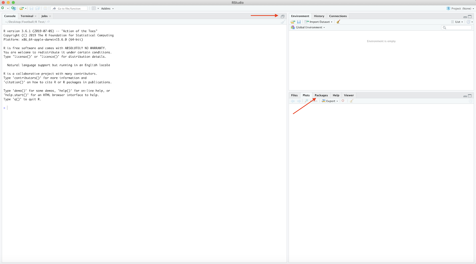
Press the arrowed areas to reveal:

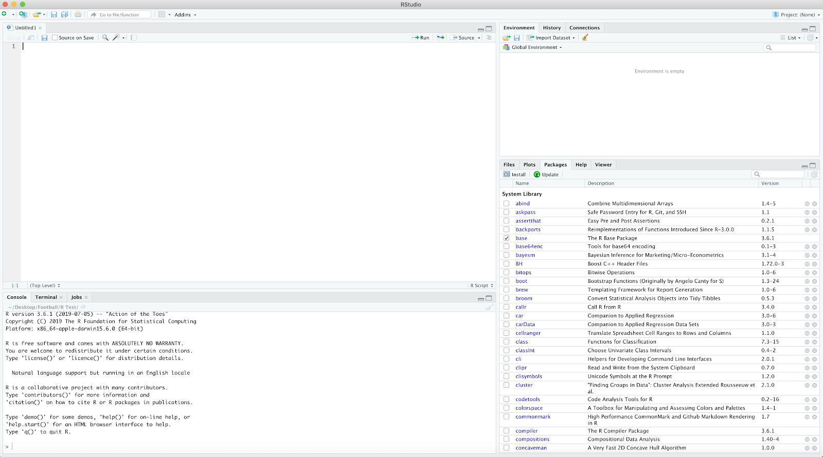
Under the packages tab select ‘Install’ and search for "devtools”. This is used to install some of the packages that will be used to work with/manipulate/plot the data.

Perform the previous once again, but this time searching for ‘tidyverse’. The tidyverse package consists of other packages that help working with data (dplyr) and visualising data (ggplot)

Finally, install Statsbomb (for the open data) and SBpitch (to plot a pitch):

devtools::install_github("statsbomb/StatsBombR")
devtools::install_github("FCrSTATS/SBpitch")

On each line just hit “run”, or if on a Mac, you can use the keyboard shortcut of command+enter - this executes the code in the editor.

Once this is installed the packages can be loaded via library()

library(StatsBombR)
library(tidyverse)
library(SBpitch)

At this point everything required is imported and ready to be used…lets move on to the fun stuff!

---

StatsbombR comes with functions that help to navigate the available data. The first of which is FreeCompetitions(). By hitting run on this, a tibble is created in the console showing the available competitions along with other information:

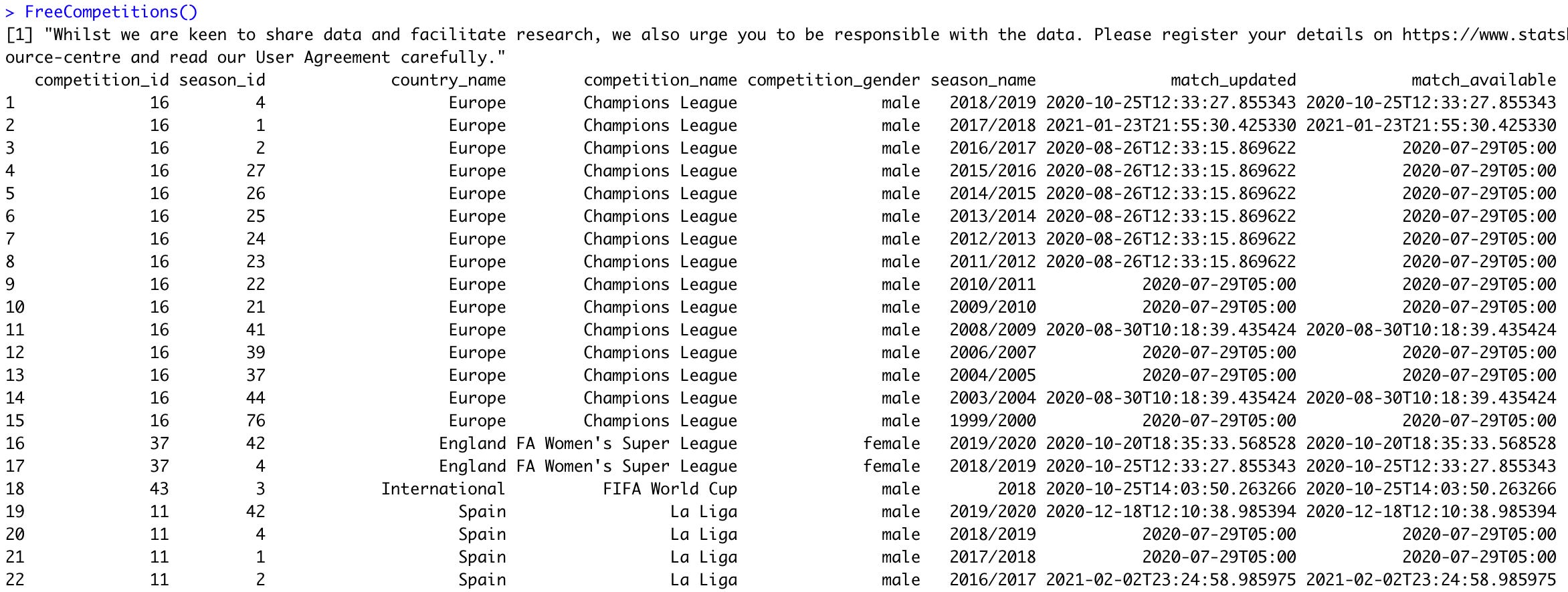
There are 37 competitions including Champions League 1999-2019, La Liga 2014-2020, NWSL and WSL. Throughout the FAWSL data for 2019/2020 will be used.

We will now ‘assign’ FreeCompetitions(), this will enable us to use the data in further steps ( to assign, ‘<-’ is used):

##load competitions
Comp<-FreeCompetitions()

view(Comp)

By running view(Comp)the previous tibble is returned as a data frame. Next step is to specify the league and season we wish to use. Tidyverse now comes in to manipulate the data, using filter():

##filter WSL(37) and season
Comp<-FreeCompetitions()%>%
  filter(competition_id==37, season_name=="2019/2020")

View(Comp)

A few things to break down in the two lines of code!

Firstly, %>% is the pipe, which essentially means: ‘and then’.

Secondly, ‘==’ refers to an exact match…other operations can be used such as:

1. > (greater than)

2. >= (greater than or equal to)

3. & (and)

4. | (or).

Therefore, in the above lines we are taking FreeCompetitions() and filtering the competition_id and season_name columns for exactly 37 and 2019/2020 respectively, before assigning to Comps. Using view(Comps) there should be a single row of information referring to the FAWSL 2019/2020 season.

The second statsbombR function to utilise is FreeMatches(). No prizes, but this will pull the available matches for a given competition:

##load available matches for WSL 2019/2020
Matches<-FreeMatches(Competitions = Comp)

view(Matches)

The above takes the competition selected earlier and finds all matches played, before assigning to ‘Matches’. You can use either view(Matches) or head(Matches) to see the outcome - 87 rows (a single row for each match) and 40 columns.

Finally, to pull the available event data for the 87 matches and clean! StatsBomb have been kind once more creating StatsBombFreeEvents() and allclean() functions:

StatsBombData<-StatsBombFreeEvents(MatchesDF = Matches, Parallel = T) %>% 
allclean()

view(StatsBombData)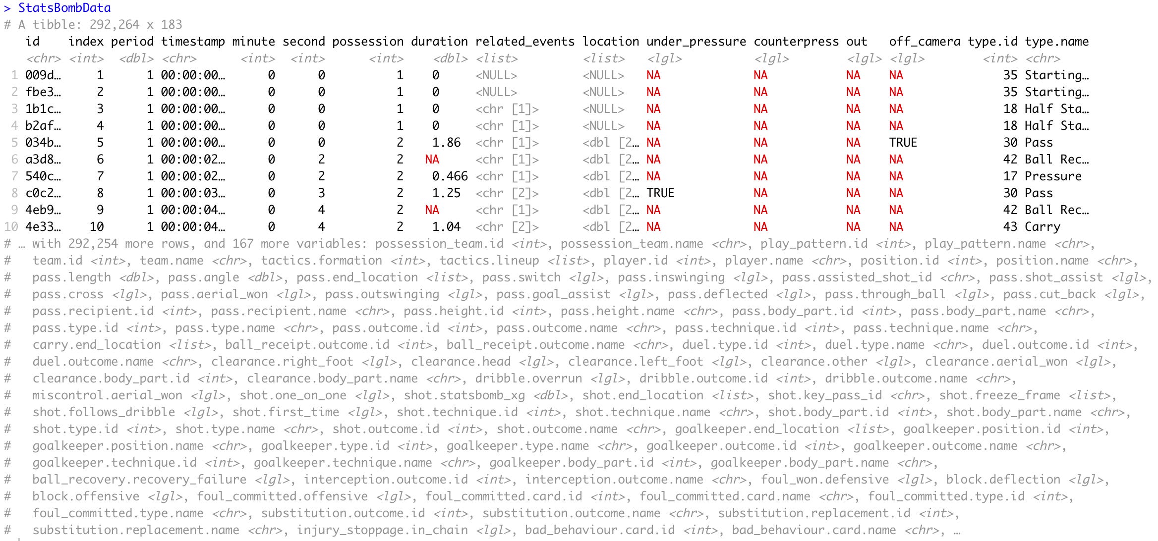

Okkkkkkkk…292,264 rows with 183 columns. At this point have a good look at the data!

We require a limited number of the 183 columns so will now select() the required columns and store within ‘data’:

##select columns
data<-StatsBombData %>%
 select(id, type.name, team.name, player.name, position.name, pass.outcome.name, match_id, location.x, location.y, pass.end_location.x, pass.end_location.y)

This becomes a little more manageable! Using unique() we can observe all match_id’s, select one, then filter so we narrow events to a single match.

##find unique match_id's
unique(data$match_id)

Selected match_id = 2275096

##filter to a single match
data<-data %>% 
  filter(match_id==2275096)

##which match selected?
unique(data$team.name)

view(data)

We appear to have selected Arsenal vs West Ham!

A chunk of code:

data<-data %>%
  filter(type.name == "Pass", 
         team.name == "Arsenal WFC") %>%
  mutate(pass.outcome = as.factor(if_else(is.na(pass.outcome.name), "Complete", "Incomplete")))

view(data)

To walk through this:

1. Selecting passes made by Arsenal WFC (filter())

2. mutate() = new column

3. pass.outcome = new column name

4. if (if_else) pass.outcome.name is “NA” (is.na) add “Complete”, if not, add “Incomplete”

If we inspect the data once more there should now be an additional column labelled ‘pass.outcome’.

All the above code could be added into a single chunk…the beauty of the pipe!

data<-StatsBombData %>%

  filter(match_id==2275096, 
         type.name == "Pass", 
         team.name == "Arsenal WFC") %>%

  mutate(pass.outcome = as.factor(if_else(is.na(pass.outcome.name), "Complete", "Incomplete"))) %>% 

  select(id, type.name, team.name, player.name, position.name, pass.outcome.name, match_id, location.x, location.y, pass.end_location.x, pass.end_location.y)

At this point the data is ready to plot (for our needs!)

Ggplot as part of the tidyverse now comes in to visualise the data. Ggplot builds in layers, therefore the pitch is plotted initially, before plotting pass start/end locations on top!

##initialise pitch plot
create_Pitch()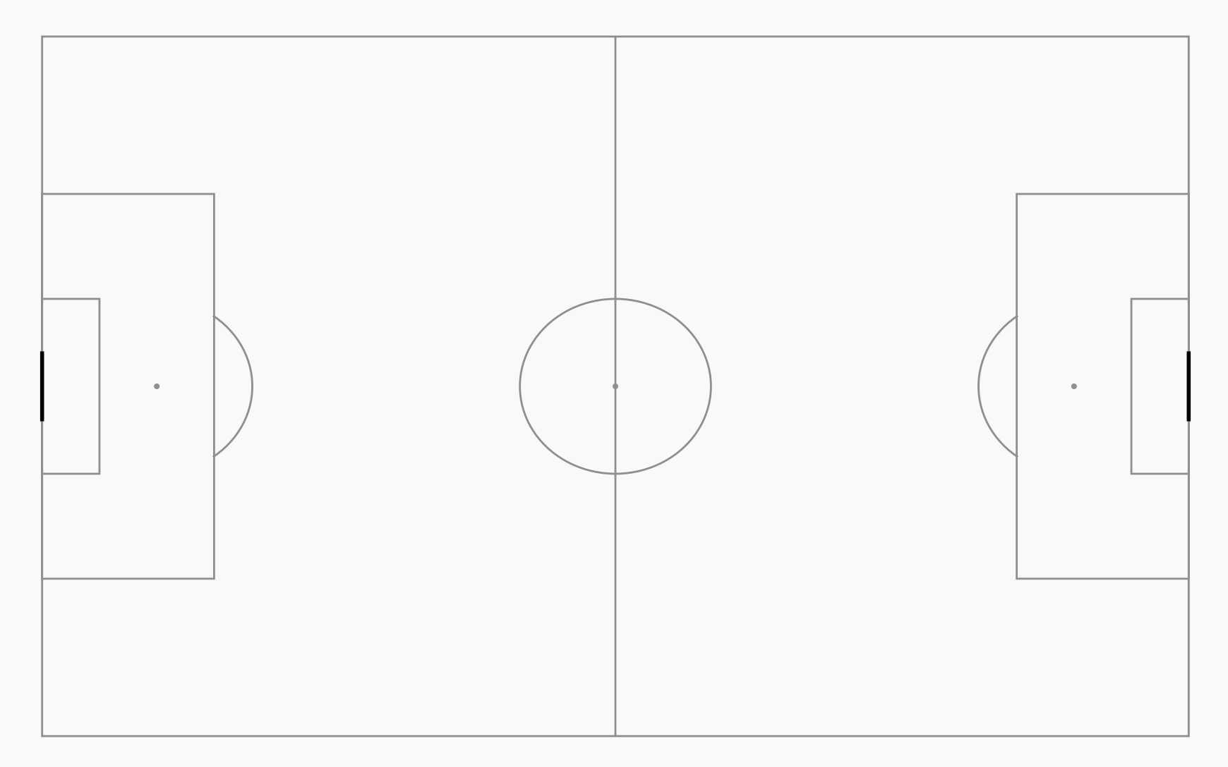

By using ?create_Pitch the documentation can be viewed - this gives an idea of the customisation that can be made within the function:

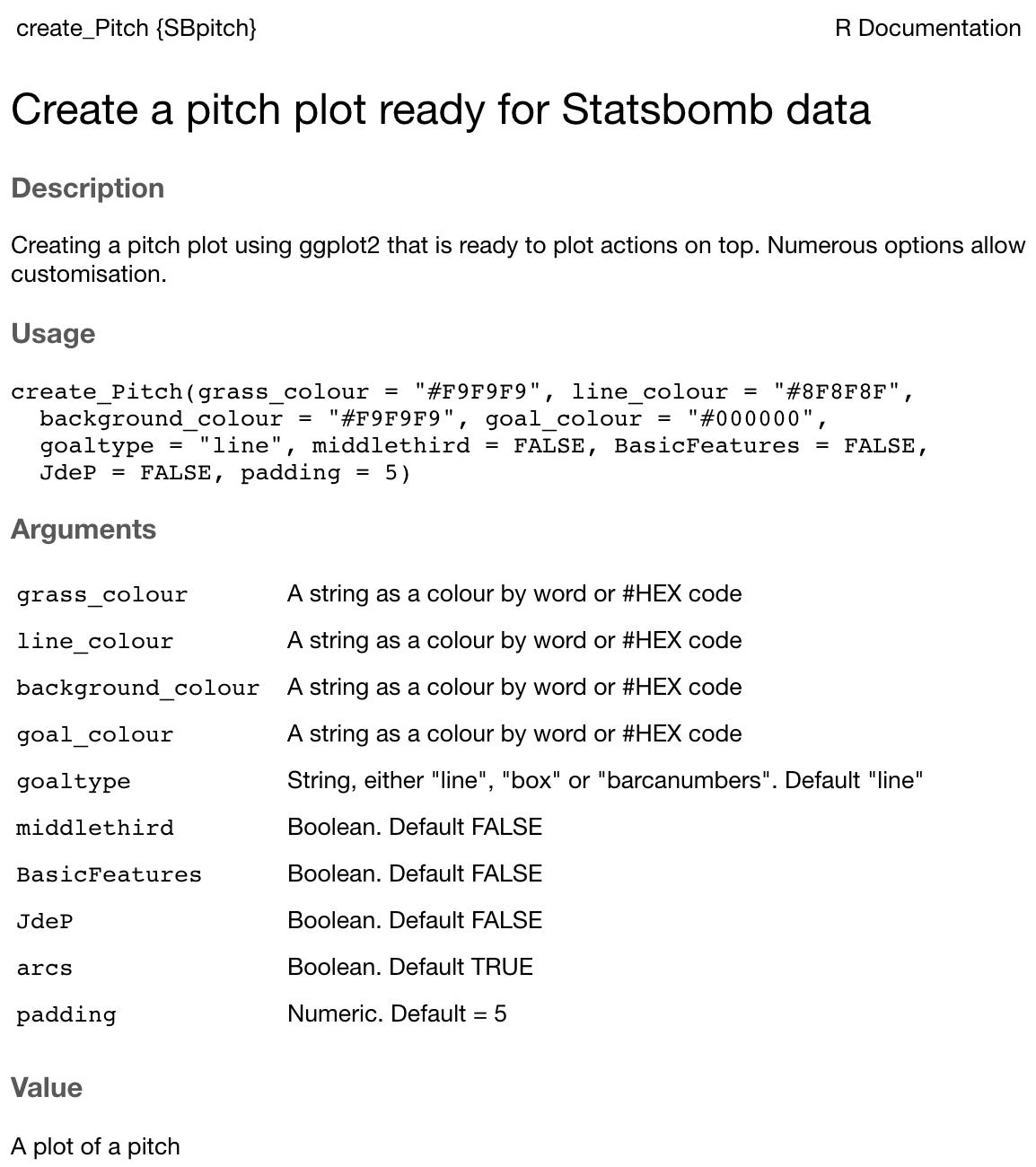
To have a quick tinker, to change the goal line type and add Juego de Posicion lines: create_Pitch(JdeP = TRUE, goaltype = "barcanumbers")

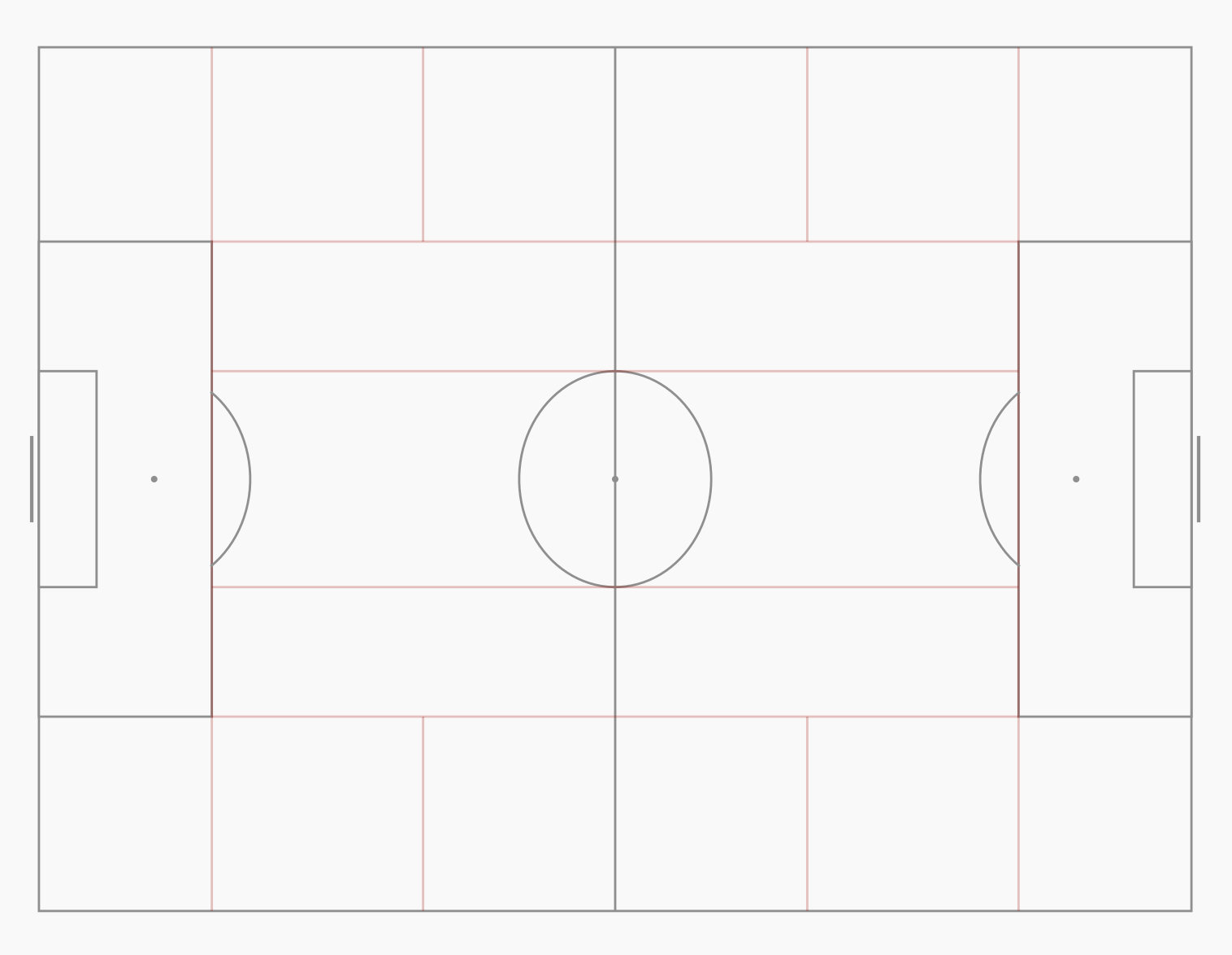
You can customise as much as you wish - I will continue with the standard base pitch.

To build on the pitch layer, the start positions of the passes can be added:

##plot pass start locations
create_Pitch()+
  geom_point(data = data, aes(x = location.x, y = location.y))

Again, looking at the documentation the transparency, colour, size can all be altered:

##customise points
create_Pitch()+
  geom_point(data = data, aes(x = location.x, y = location.y), colour = "red", alpha = 0.7)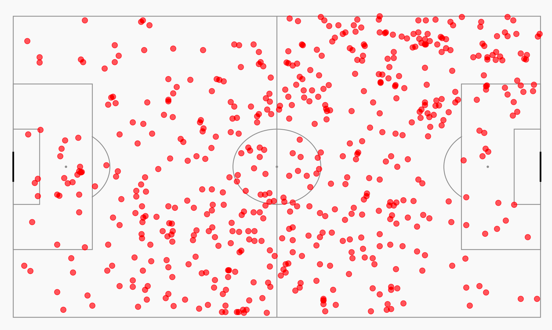

Now to see where passes start and end, adding an arrow using geom_segment() and flip the y axis.

create_Pitch()+

  geom_point(data = data, aes(x = location.x, y = location.y), alpha = 0.5)+

  geom_segment(data = data, aes(x = location.x, y = location.y, xend = pass.end_location.x, yend = pass.end_location.y), alpha = 0.5, arrow = arrow(length = unit(0.06,"inches"))) +

scale_y_reverse()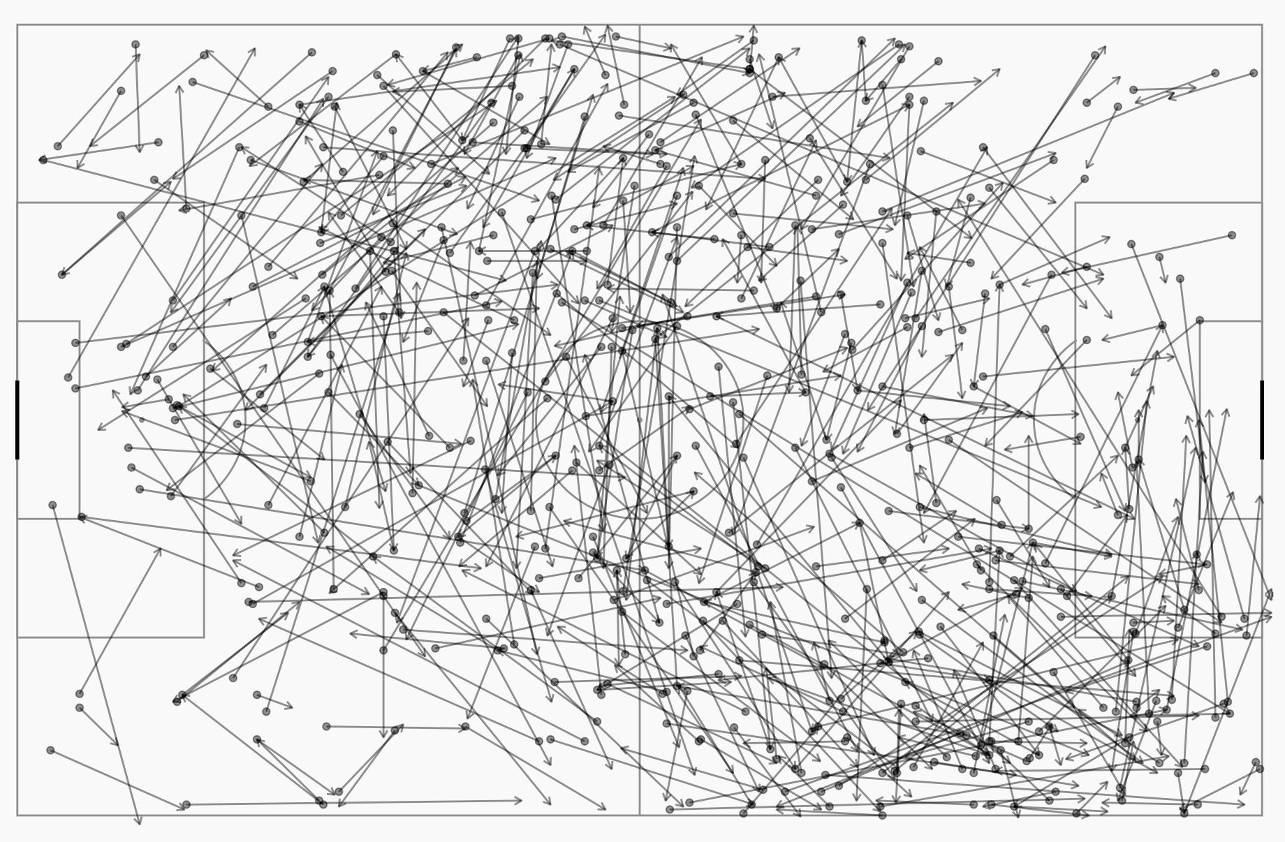

Lovely stuff. This starts to provide some insight, but would be handy to to know the pass outcomes - the pass.outcome column that was created earlier now comes into play!

create_Pitch()+

  geom_point(data = data, aes(x = location.x, y = location.y, colour = pass.outcome), alpha = 0.5)+

  geom_segment(data = data, aes(x = location.x, y = location.y, xend = pass.end_location.x, yend = pass.end_location.y, colour = pass.outcome), alpha = 0.5, arrow = arrow(length = unit(0.06,"inches"))) +

  scale_y_reverse()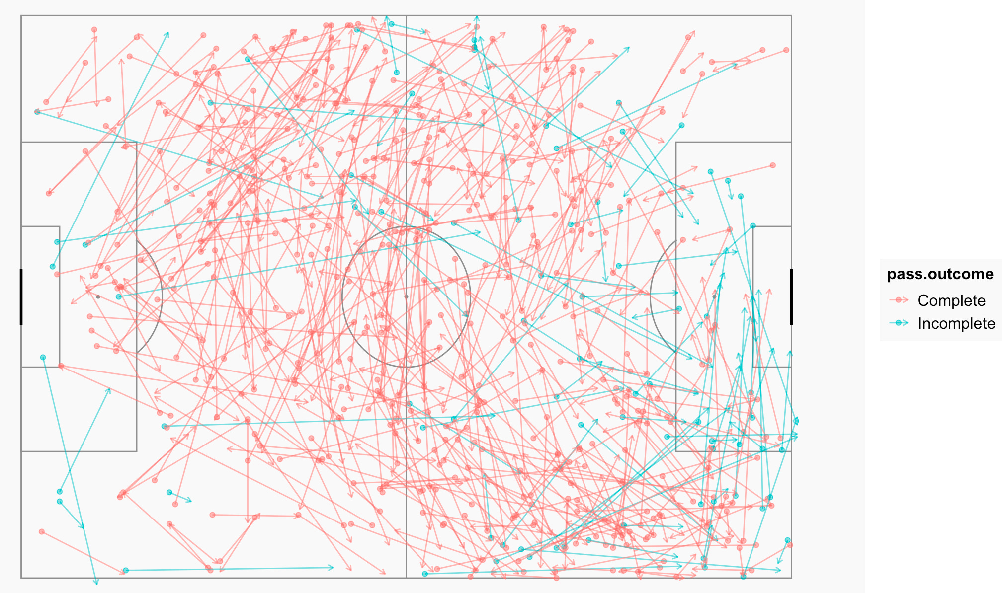

Adding the outcome colour to aes()within geom_point() and geom_segment() creates the legend - I will slightly change this to flip the colours:

create_Pitch()+

  geom_point(data = data, aes(x = location.x, y = location.y, colour = pass.outcome), alpha = 0.5)+

  geom_segment(data = data, aes(x = location.x, y = location.y, xend = pass.end_location.x, yend = pass.end_location.y, colour = pass.outcome), alpha = 0.5, arrow = arrow(length = unit(0.06,"inches"))) +

  scale_y_reverse()+

  scale_color_manual(values = c("#00b0f6", "#f8766d"), name = "Pass Outcome")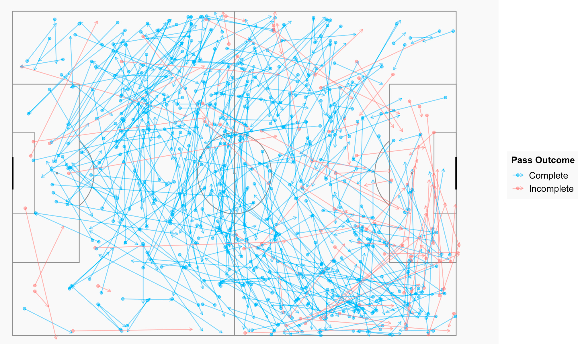

Final part! Adding a title/subtitle/caption:

##Plot!
create_Pitch()+

  geom_point(data = data, aes(x = location.x, y = location.y, colour = pass.outcome), alpha = 0.5)+

  geom_segment(data = data, aes(x = location.x, y = location.y, xend = pass.end_location.x, yend = pass.end_location.y, colour = pass.outcome), alpha = 0.5, arrow = arrow(length = unit(0.06,"inches"))) +

  scale_y_reverse()+

  scale_color_manual(values = c("#00b0f6", "#f8766d"), name = "Pass Outcome")+

  labs(title = "Arsenal WFC Passes",
       subtitle = "vs West Ham United LFC",
       caption = "Data: StatsBomb | by: @biscuitchaser")+
  
  ##use theme() to adjust aesthetics
  theme(plot.title = element_text(size = 30, hjust = 0.5, face = "bold"),
        plot.subtitle = element_text(size = 15, hjust = 0.5),
        plot.caption = element_text(size = 12, face = "bold"))

Once the title and subtitle are added, they can be adjusted within theme(). Plot.title() refers to the title with the font size, font face and title position (hjust) altered, giving the result:

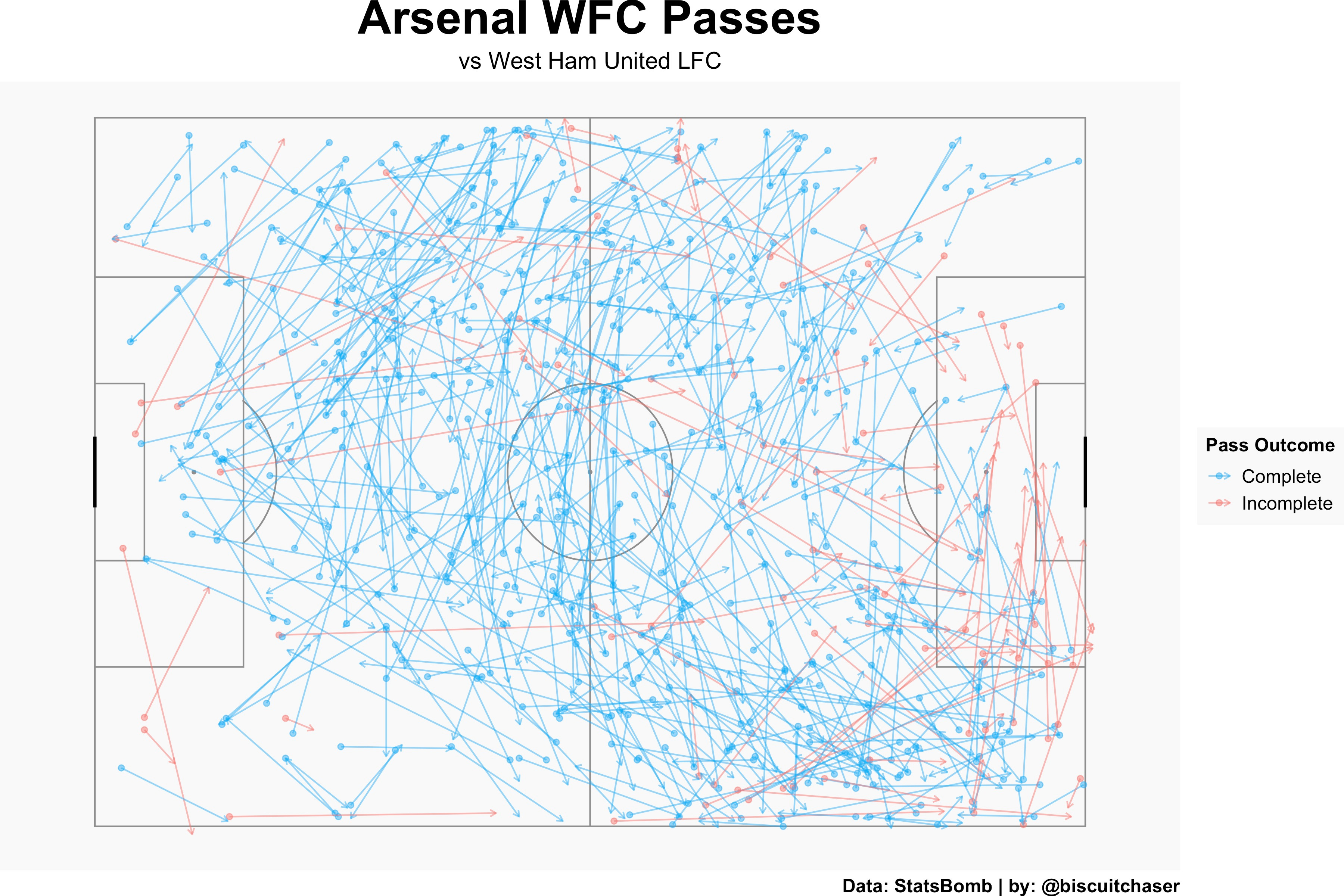
Great! Finally to save:

ggsave(plot = last_plot(), filename = "arsenal_vs_westham.jpg", height = 8, width=12)

You should now have saved the above image with the filename ‘arsenal_vs_westham’

Job done! You can have a play filtering by different matches/teams/players. Personally, I seem to learn through trial and error, breaking and fixing things - this may not apply to everyone!

As always, let me know if you have any issues/questions - I hope this has been a logical walk through getting started with R using StatsBomb data!

---

library(StatsBombR)
library(tidyverse)
library(SBpitch)

##load competitions and filter by WSL 2019/2020 - FreeCompetitions() will load availble competitions including WSL/Spain/Champions League
Comp<-FreeCompetitions()%>%
  filter(competition_id==37, season_name=="2019/2020")

##load available matches for WSL 2019/2020
Matches<-FreeMatches(Competitions = Comp)

##load events for above matches
StatsBombData<-StatsBombFreeEvents(MatchesDF = Matches, Parallel = T) %>% 
  allclean()

##clean data
StatsBombData = allclean(StatsBombData)

##filter events data to select match_id and all passes - create new "complete"/"incomplete" variable
data<-StatsBombData %>%
  filter(match_id==2275096, 
         type.name == "Pass" & is.na(pass.type.name), 
         team.name == "Arsenal WFC") %>%
  mutate(pass.outcome = as.factor(if_else(is.na(pass.outcome.name), "Complete", "Incomplete")))


##Plot!
create_Pitch()+

  geom_point(data = data, aes(x = location.x, y = location.y, colour = pass.outcome), alpha = 0.5)+

  geom_segment(data = data, aes(x = location.x, y = location.y, xend = pass.end_location.x, yend = pass.end_location.y, colour = pass.outcome), alpha = 0.5, arrow = arrow(length = unit(0.06,"inches"))) +

  scale_y_reverse()+

  scale_color_manual(values = c("#00b0f6", "#f8766d"), name = "Pass Outcome")+

  labs(title = "Arsenal WFC Passes",
       subtitle = "vs West Ham United LFC",
       caption = "Data: StatsBomb | by: @biscuitchaser")+
  
  ##use theme() to adjust aesthetics
  theme(plot.title = element_text(size = 30, hjust = 0.5, face = "bold"),
        plot.subtitle = element_text(size = 15, hjust = 0.5),
        plot.caption = element_text(size = 12, face = "bold"))

ggsave(plot = last_plot(), filename = "arsenal_vs_westham.jpg", height = 8, width=12)